In our use of analog sensors (sensors that produce a voltage that we measure using the analog-to-digital converter connected to pins A0 to A7) we had to deal with noise. If the sensor did not produce a strong enough signal, the noise overwhelmed it, and the readings varied a lot. We used averaging to get a better idea of the real signal, at the expense of time, memory, and program complexity.
But there are other ways to measure things like light and temperature that do not use the A/D converter, and are less sensitive to analog noise (although they may have other kinds of noise). They may have other advantages, like higher resolution (more than 1024 discrete levels), also known as higher dynamic range.
Let's take another look at our LED light sensor. When we used it as a photocell, it produced a voltage from 0 to 1.4 volts, depending on the light. The 10 bit analog to digital converter in the tiny computer using the 5 volt default reference voltage, would see the highest brightness as 1.4 volts divided by 5. Since 10 bits means a range of 2 to the tenth power, or 1024, the highest light level would be a reading of 1.4 * 1024 / 5, or 286. So our resolution was 1 part in 286. That's just a little bit over 8 bits (2 to the eighth power is 256).
We could get better results using the 3.3 volt reference. Then we would have 1.4 * 1024 / 3.3, or 434. That is just shy of 9 bits of resolution (2 to the ninth power is 512).
But there is a way to get over 14 bits of resolution. We can measure light to one part in 18,000 or even more.
The trick is to recognize that an LED is also a capacitor. A capacitor is just two conductors separated by an insulator. The two legs of the LED are conductors, and the material between them is a semiconductor. A semiconductor can look like an insulator or a conductor, depending on the electrical charges in it. If our LED is in the dark, there is no light to generate electric charges, so it is more of an insulator. If it is in bright light, there are lots of charges generated, and it becomes less of an insulator.
A capacitor stores electric charge. If we put 5 volts on one pin, and zero volts on the other, electrons will build up on one side but not the other. We say the capacitor is charged when no more electrons can be pushed onto that side. If we connect the two leads, electrons can flow from one side to the other, until both sides are equal. We then say the capacitor isdischarged. As a capacitor is discharging, the current flowing through the connection can perform work, such as lighting a light, or running a motor. In this way a capacitor is similar to a rechargeable battery.
If we have the tiny computer charge the capacitance of the LED to 5 volts, we can time how long it takes for the charge to drain away, due to how well the semiconductor acts as an insulator. In the dark, it will take a long time to drain. In the light, it will drain quickly.
We can do this timing by counting in a loop. The program to do this is here.
We connect the LED between pins 2 and 3 of the tiny computer. The long leg of the LED (the anode) is connected to pin 3. The shorter leg is connected to pin 2.

If we set pin 2 to LOW (zero volts) and pin 3 to HIGH (5 volts) the LED will light up. But we don't want that. We do the opposite. We set pin 2 to HIGH, and pin 3 to LOW. That charges our LED capacitor.
Now we set pin 2 to be an input instead of an output. This way it will read the voltage on the LED capacitor as either a 0 bit (meaning the voltage has dropped to below 2.6 volts), or a 1 bit (meaning it is 2.6 volts or higher). We also have to write a LOW value to the pin, to disconnect an internal resistor that otherwise tries to raise the pin to 5 volts. We'll talk more about pull-up resistors and why they are there later.
The code then loops, checking to see if the voltage has dropped below 2.6 volts. As it loops, it counts, using the variable level. When the pin reads as a 0 bit, we return the value of level. This gets printed on the USB serial port.
In the dark, we can see the loop takes over 18,000 iterations before the pin reads as a zero bit. In very bright light, it only takes 30 or so iterations through the loop.
Noise
While we have successfully expanded the dynamic range of our measurement, there is still quite a bit of noise in the signal. The tiny LED still has a high impedance, and it cannot produce enough power to overwhelm variations in the computer's power supply and other sources of noise. One important source of noise in this case is radio waves from nearby WiFi access points, microwave ovens, and cell phones, as well as more distant television and radio transmitters, and sparks from electric motors. To reduce this, we have put the LED as close to the tiny computer as possible. When we had longer leads (to make it easier to put the sensor in the dark), we noticed that merely bringing a hand near the wires was enough to significantly change the values reported in the output.
A Comparison
If both our light sensors seem to have a fair bit of noise, can we tell if one is better than the other?
The noise is what the standard deviation measures. The mean is what we call the signal. If we divide the mean by the standard deviation, we get something called the signal to noise ratio, or SNR. So if we take a set of readings using one light sensor, and another set using the other light sensor, we can calculate the signal to noise ratio for each one, and then compare them to see which is better.
The connections to the LEDs are the same as before. We added a bit of black electrician's tape to cover the on-board LEDs so they would not flicker and interfere with the readings:

The code to do this is here.
The bulk of the code is not new. It is a copy the code for each of the two types of light sensor. But we have added a new class to make calculating the statistics simpler and better.
When we first started calculating the mean and the standard deviation, we collected the samples into an array, calculating the mean as we went. Then we made a second pass through the array, calculating the sum of squared differences from the mean (the variance).
But by doing a little rearranging of the math, we can avoid the array, and the second pass through the data, and calculate the mean and the standard deviation as we encounter each sample. Avoiding the array means that we are no longer limited by the small memory in the tiny computer, and we can collect tens of thousands of samples, or many more.
The class that does this is shown below:
class Stats
{
unsigned long n;
double mean;
double variance;
double sum;
public:
Stats( void )
{
n = 0; mean = 0; variance = 0; sum = 0;
}
void sample( double s )
{
double delta = s - mean;
n++;
mean += delta / n;
sum += delta * delta;
}
double get_mean( void ) { return mean; }
double get_variance( void ) { return sum / n; }
double get_sd( void ) { return sqrt( sum / n ); }
double get_snr( void ) { return get_mean() / get_sd(); }
};
;
The constructor sets all the class variables to zero. The sample() method is what does all the work.
For each sample, we calculate the difference between it and the current mean, and we increment the sample count.
Then we add to the mean this difference, divided by the current sample number.
Lastly, we add the squared difference into the running total.
The remainder of the class are methods that return the values we are interested in.
The program declares two instances of the Stats class:
Stats digital_stats;
Stats analog_stats;
to collect the data for the two different sensors.
In the loop() function, the sample() method is called for each sample from each sensor:
digital_stats.sample( digital );
analog_stats.sample( analog );
Then the results are printed out:
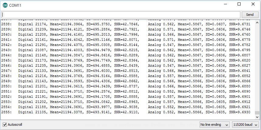
As we would expect, as the sample size grows, our uncertainty (the standard deviation) tends to get smaller, and our signal to noise tends to get bigger. But what we want to see is which sensor has the better signal to noise ratio. For my sensors, the digital one wins by a factor of four.
It is interesting to play a flashlight over the sensors and watch as the SNR changes. If one sensor is seeing more light variation than the other (because holding the flashlight still is not easy), you will see that variation show up in the SNR reading.